ICRA 2026 BARN Challenge: NMPC Navigation on the Jackal
Team Robo's NMPC navigation stack (acados, Clearpath Jackal) for the ICRA 2026 BARN Challenge: 3rd place in the physical finals in Vienna.
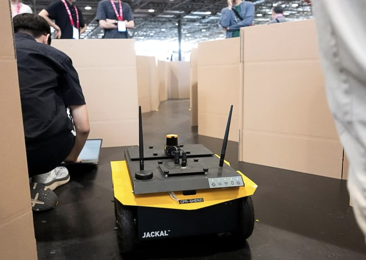
The BARN (Benchmark Autonomous Robot Navigation) Challenge asks teams to drive a Clearpath Jackal through dense, narrow obstacle courses as fast as possible without touching anything. The robot has a single 270° 2D LiDAR and a 2 m/s top speed. I led Team Robo from NTU (8 members) in the 2026 edition, held at ICRA 2026 in Vienna.
| Stage | Result |
|---|---|
| Simulation (17 teams) | 6th, score 0.4515, invited to the physical finals |
| Physical finals, Vienna, 2–4 June 2026 | 3rd place, 3 of 9 trials successful |
| Dynamic-environment benchmark | 1st all-time |
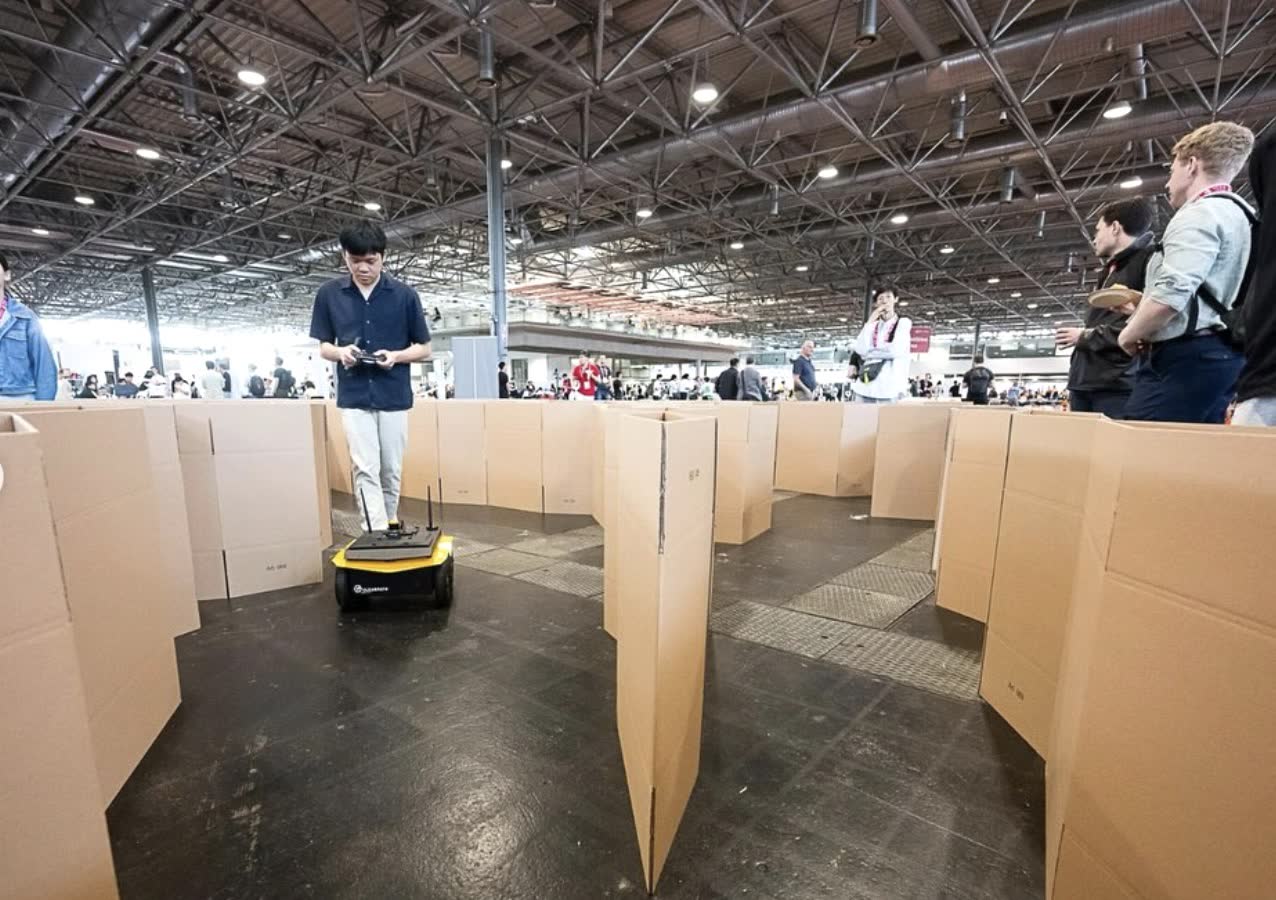 Physical finals at the Vienna Congress & Convention Center. The course is built from cardboard boxes and changes between rounds.
Two runs from the physical final
Left: trial 1. Right: trial 2. The Jackal runs fully autonomously on its 2D LiDAR through the cardboard course.
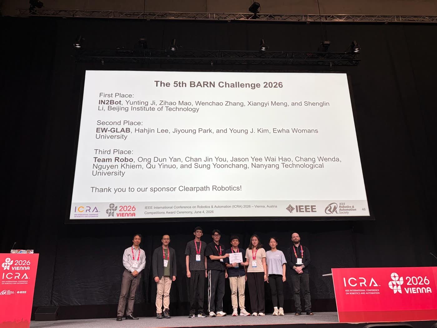 Award ceremony at ICRA 2026, Vienna: Team Robo from NTU in third place.
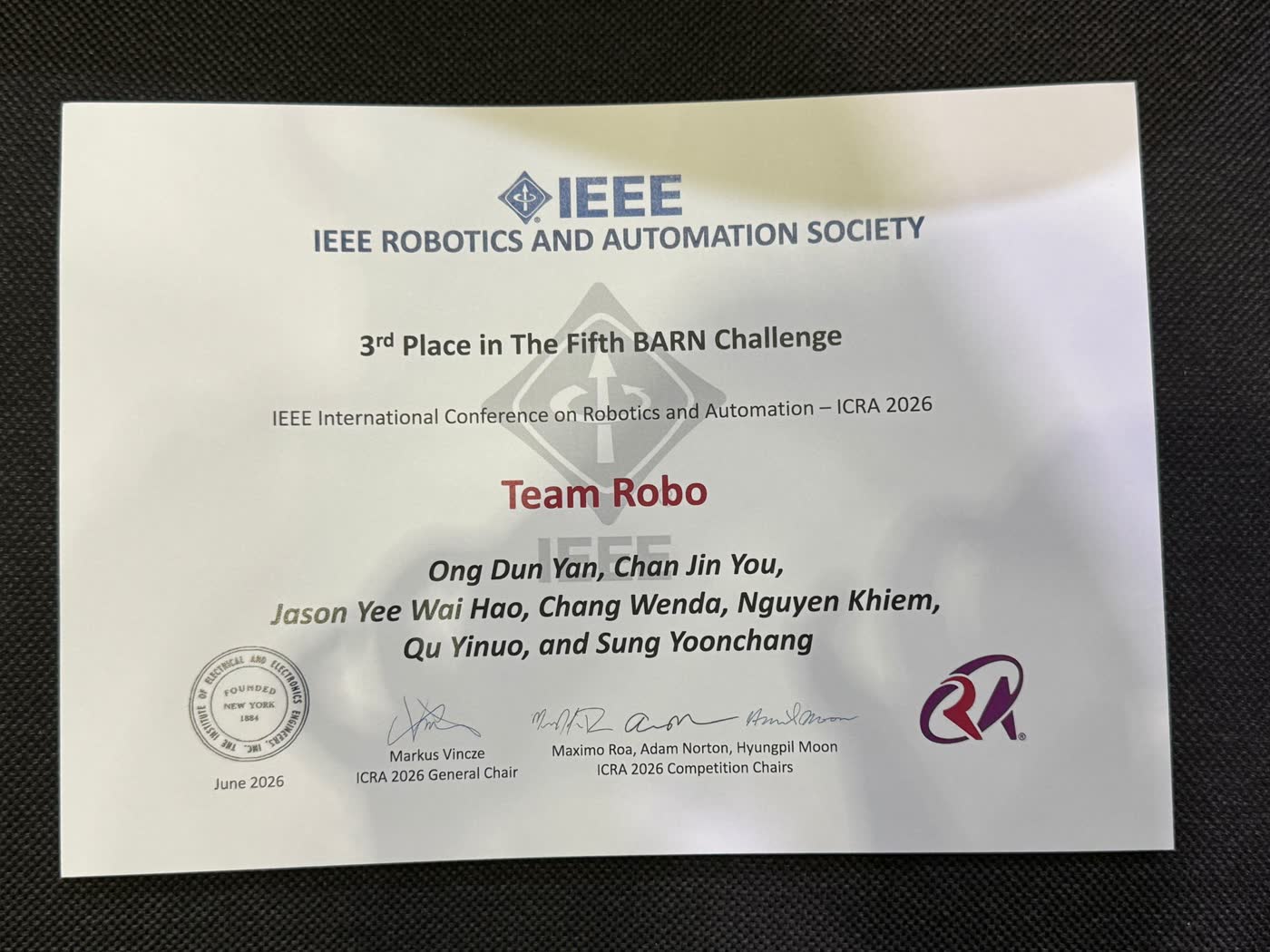 The IEEE Robotics and Automation Society certificate for 3rd place.
Approach: one NMPC, several modes
Most BARN stacks are tuned for static clutter. We built a nonlinear model predictive controller (NMPC) that can handle static walls and moving obstacles in the same optimisation, solved in real time with acados. Many times a second it plans a short stretch of motion ahead, applies the first step, and plans again.
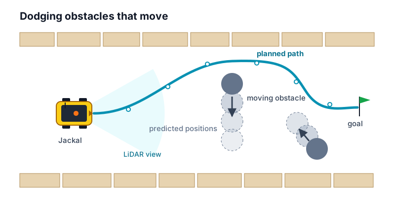 The idea in one picture: moving obstacles are tracked, their future positions predicted, and the planned path bends around where they will be, not where they are.
The robot model
The Jackal is a differential-drive robot. We model its two wheel speeds directly, so the controller respects how quickly the real wheels can speed up and slow down:
\[\begin{gathered} v = \frac{v_r + v_l}{2}, \qquad \omega = \frac{v_r - v_l}{L} \\[6pt] \dot x = v\cos\theta,\quad \dot y = v\sin\theta,\quad \dot\theta = \omega \end{gathered}\]The optimisation, in words
\[\begin{gathered} \min_{\text{controls}}\; \underbrace{\text{tracking error}}_{\text{stay on the path}} + \underbrace{\text{control effort}}_{\text{move smoothly}} \\[8pt] \text{subject to}\quad \underbrace{\text{robot limits}}_{\text{speed, turning}},\;\; \underbrace{\text{clearance}}_{\text{now and predicted}} \end{gathered}\]The clearance constraints are soft: in a gap tighter than the safety margin, the solver may give up a little clearance at a high cost instead of failing outright. In a course as tight as BARN, that difference matters.
Modes: same solver, different priorities
The repository is called mode-switching MPC because the controller changes what it prioritises depending on the situation. The optimisation stays the same; each mode adjusts what it is asked to do.
flowchart LR
  S{"Moving obstacle<br/>nearby?"} -- yes --> D[Dynamic]
  S -- no --> G{"Goal close<br/>and clear?"}
  G -- yes --> R[Rush to goal]
  G -- no --> W{"Walls close?"}
  W -- yes --> T[Static]
  W -- no --> N[Normal]
- Normal: open space, go fast.
- Static: tight walls, move carefully.
- Dynamic: something is moving nearby, plan around where it is heading.
- Rush to goal: the finish is close and clear.
- When the path doubles back, the robot can also turn on the spot or reverse out instead of attempting a wide turn.
Tracking moving obstacles
The moving obstacles come from our obstacle tracker, built on Mateusz Przybyła’s obstacle_detector. It turns the laser scan into shapes and follows them over time to estimate how fast each one is moving.
A raw tracker reports everything, including walls that only seem to move because of sensor noise. We added a filter so that only genuinely moving obstacles reach the controller, which stops the robot from swerving around phantoms.
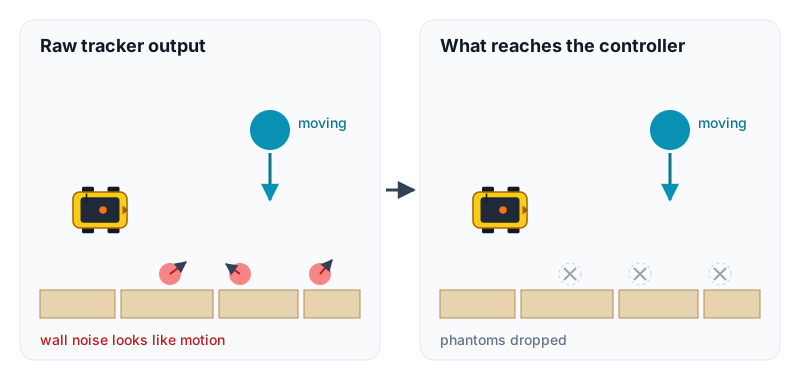 Left: the raw tracker sees “motion” in wall noise. Right: after our filter, only the real moving obstacle is passed on.
Simulation vs. the physical finals
The work lives in two branches of the repository:
v3.0, simulation: the full stack including moving-obstacle tracking, used for the dynamic benchmark.main, physical finals: the version that ran in Vienna. The 2026 courses were static, so tracking was switched off. It is packaged as a standardmove_baseplugin and hardened for real sensor noise.
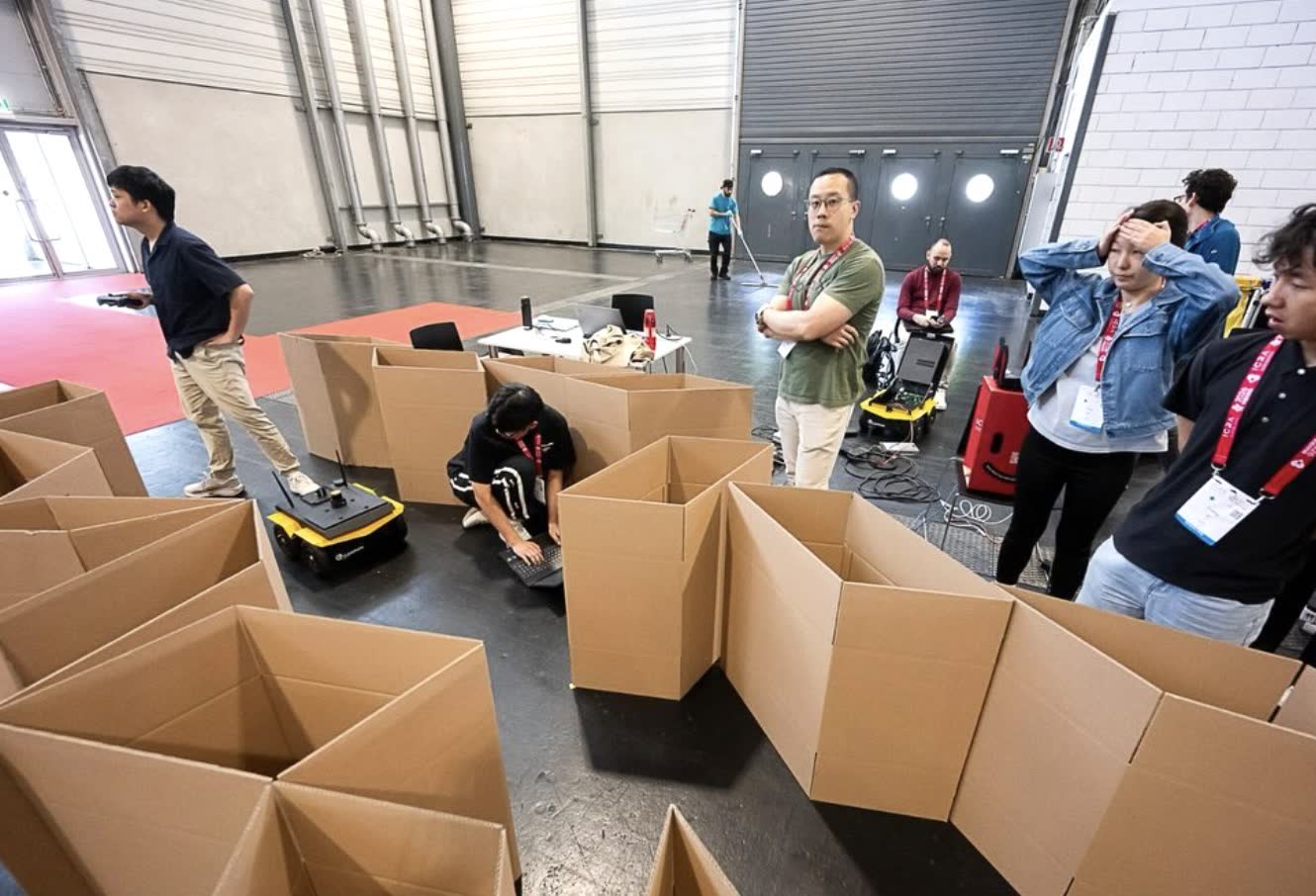 Setting up between trials. Each team gets a fixed time slot per course.
Context from the finals
- Simulation and physical rankings differed. Only four of the seven invited teams competed in Vienna, and the order changed: we placed 6th in simulation and 3rd on the real robot.
- The 2026 courses were static only. Unlike earlier editions, there was no dynamic-obstacle component. Our dynamic handling went unused in the finals, but it is what ranks us first all-time on the dynamic-environment benchmark.
- Every team in the finals used classical methods. For the second year in a row, no finalist used machine learning in their navigation stack.
Our approach is described in the organisers’ article on the competition: Autonomous Ground Navigation in Highly Constrained Spaces: Lessons Learned from the Fifth BARN Challenge at ICRA 2026, submitted to IEEE Robotics and Automation Magazine.
My role
- Led the 8-member team through the simulation qualifier and the physical finals.
- Wrote most of the mode-switching MPC planner (C++, acados, ROS
move_baseplugin). - Co-developed the laser-based dynamic obstacle tracker, including the filter that keeps only genuinely moving obstacles.
- Also built and tested alternative planners we compared against: a D* Lite global planner, a visibility-graph global planner, and DDP-based local planning.